

It's the basic encoding for analog TV. It is used in the NTSC and PAL. The luminance Y is compute as:
The components U and V are the difference between red or blue and the luminance weighted by a fator.
et
We can also write this conversion in the following way:
The inverse transformation YUV to RGB is compute as:
The Matlab program :
% conversion RGB --> YUV

%normalisation des couleurs

Y = 0.299*R + 0.587*G + 0.114*B  ;

U = 0.492*(B-Y);

V = 0.877*(R-Y);

Rp= Y + 1.140*V;

Gp= Y - 0.395*U -0.581*V;

Bp= Y + 2.032*U ;

figure(  'Name','RGB --> YUV',...

            'NumberTitle','off',...

            'color',[0.3137 0.3137 0.5098]);

vide=zeros(ligne,colonne);

subplot(331)

imshow(uint8(cat(3,R,vide,vide)))

title('Image R origine')

subplot(334)

imshow(uint8(cat(3,vide,G,vide)))

title('Image G origine')

subplot(337)

imshow(uint8(cat(3,vide,vide,B)))

title('Image B origine')

subplot(332)

imagesc(Y,[min(min(Y)) max(max(Y))])

colormap(gray)

axis image

title('Image Y')

subplot(335)

imagesc(U,[min(min(U)) max(max(U))])

colormap(gray)

axis image

title('Image U')

subplot(338)

imagesc(V,[min(min(V)) max(max(V))])

colormap(gray)

axis image

title('Image V')

subplot(333)

imshow(uint8(cat(3,Rp,vide,vide)))

title('Image R reconstruit')

subplot(336)

imshow(uint8(cat(3,vide,Gp,vide)))

title('Image G reconstruit')

subplot(339)

imshow(uint8(cat(3,vide,vide,Bp)))

title('Image B reconstruit')
An example: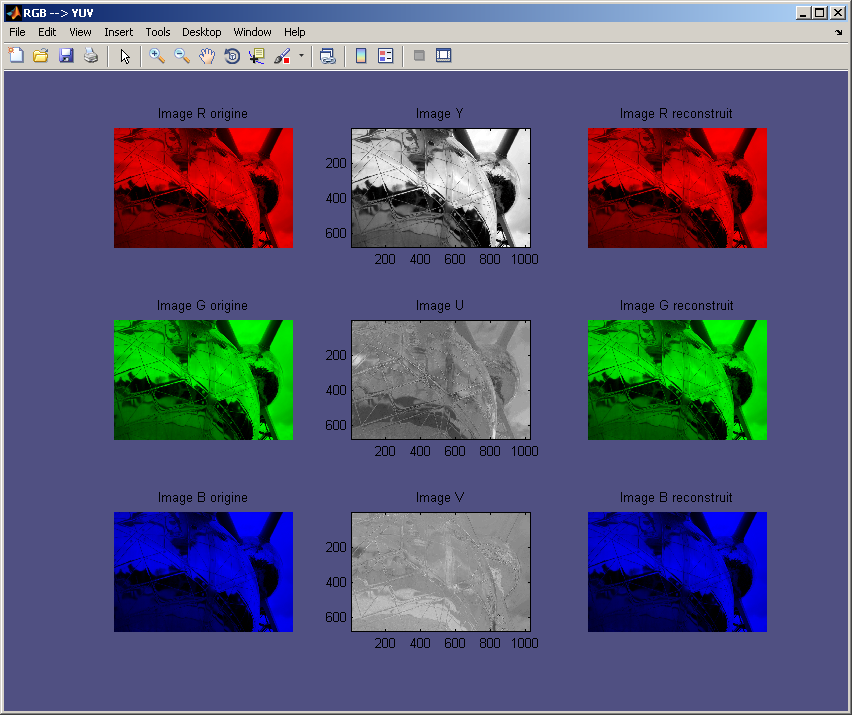
It's the original NTSC system. The luminance Y is the same as for th YUV. I represent the inphase and Q the quadrature. U and V are rotated and mirrored thanks to the angle b. Here is the equations:
et
the angle b is equal to 0.576 or 33°.
We can also compute this transformation as:
The inverse transformation is made with:
The Matlab program:
Y = 0.299*R + 0.587*G + 0.114*B  ;

U = 0.492*(B-Y);

V = 0.877*(R-Y);

b=0.576;

I = -sin(b)*U + cos(b)*V ;

Q = cos(b)*U + sin(b)*V ;

Rp= Y +  0.956*I +  0.621*Q;

Gp= Y -  0.272 *I - 0.647*Q;

Bp= Y -  1.106*I + 1.703*Q;


figure(  'Name','RGB --> YIQ',...

            'NumberTitle','off',...

            'color',[0.3137 0.3137 0.5098]);

vide=zeros(ligne,colonne);

subplot(331)

imshow(uint8(cat(3,R,vide,vide)))

title('Image R')

subplot(334)

imshow(uint8(cat(3,vide,G,vide)))

title('Image G')

subplot(337)

imshow(uint8(cat(3,vide,vide,B)))

title('Image G')

 subplot(332)

imagesc(Y,[min(min(Y)) max(max(Y))])

colormap(gray)

axis image

title('Image Y')

subplot(335)

imagesc(I,[min(min(I)) max(max(I))])

colormap(gray)

axis image

title('Image I')

subplot(338)

imagesc(Q,[min(min(Q)) max(max(Q))])

colormap(gray)

axis image

title('Image Q')

subplot(333)

imshow(uint8(cat(3,Rp,vide,vide)))

title('Image R reconstruit')

subplot(336)

imshow(uint8(cat(3,vide,Gp,vide)))

title('Image G reconstruit')

subplot(339)

imshow(uint8(cat(3,vide,vide,Bp)))

title('Image B  reconstruit')
An example: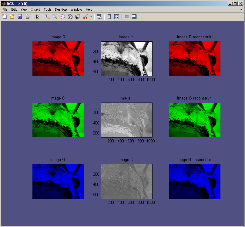
This color scale is a international standard of YUV. It is used in the digital TV and in compression (JPEG). We have for the RGB to YCbCr transformation:
where wr = 0.299, wb = 0.114 and Wc = 1 - wb - wr.
The inverse transformation YCbCr to RGB is made thanks to:
This transfomartion can also be made with the folowing matrix:
The Matlab program:
% conversion RGB --> YCbCr

%normalisation des couleurs

Wr=0.299;Wb=0.114; Wg=1-Wr-Wb;

Y = Wr*R + Wg*G + Wb*B  ;

Cb= ( 0.5 / ( 1-Wb) ) * (B-Y);

Cr= ( 0.5 / ( 1-Wr) ) * (R-Y);

Rp= Y + ((1 - Wr)/0.5)*Cr;

Gp= Y + (Wb*(1-Wb)*Cb - Wr*(1-Wr)*Cr)/(0.5*(1-Wb-Wr));

Bp= Y + ((1 - Wb)/0.5) * Cb;


figure(  'Name','RGB --> YCbCr',...

            'NumberTitle','off',...

            'color',[0.3137 0.3137 0.5098]);

vide=zeros(ligne,colonne);

subplot(331)

imshow(uint8(cat(3,R,vide,vide)))

title('Image R origine')

subplot(334)

imshow(uint8(cat(3,vide,G,vide)))

title('Image G origine')

subplot(337)

imshow(uint8(cat(3,vide,vide,B)))

title('Image B  origine')

 subplot(332)

imagesc(Y,[min(min(Y)) max(max(Y))])

colormap(gray)

axis image

title('Image Y')

subplot(335)

imagesc(Cb,[min(min(Cb)) max(max(Cb))])

colormap(gray)

axis image

title('Image Cb')

subplot(338)

imagesc(Cr,[min(min(Cr)) max(max(Cr))])

colormap(gray)

axis image

title('Image Cr')

subplot(333)

imshow(uint8(cat(3,Rp,vide,vide)))

title('Image R reconstruit')

subplot(336)

imshow(uint8(cat(3,vide,Gp,vide)))

title('Image G reconstruit')

subplot(339)

imshow(uint8(cat(3,vide,vide,Bp)))

title('Image B  reconstruit')
An example: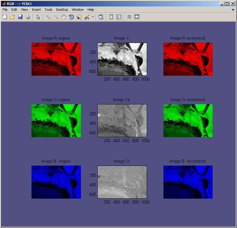
clear all;

close all;


[filename, pathname] = uigetfile({'*.jpg;*.tif;*.png;*.gif;*.bmp','All Image Files';...

          '*.*','All Files' },'mytitle',...

          'C:\Work\myfile.jpg');


img = imread(filename);

[ligne colonne dimension]=size(img);

img=double(img);

R=img(:,:,1);

G=img(:,:,2);

B=img(:,:,3);

Imax = max(max(img));


% conversion RGB --> YUV

Y = 0.299*R + 0.587*G + 0.114*B  ;

U = 0.492*(B-Y);

V = 0.877*(R-Y);

Rp= Y + 1.140*V;

Gp= Y - 0.395*U -0.581*V;

Bp= Y + 2.032*U ;

figure(  'Name','RGB --> YUV',...

            'NumberTitle','off',...

            'color',[0.3137 0.3137 0.5098]);

vide=zeros(ligne,colonne);

subplot(331)

imshow(uint8(cat(3,R,vide,vide)))

title('Image R origine')

subplot(334)

imshow(uint8(cat(3,vide,G,vide)))

title('Image G origine')

subplot(337)

imshow(uint8(cat(3,vide,vide,B)))

title('Image B origine')

subplot(332)

imagesc(Y,[min(min(Y)) max(max(Y))])

colormap(gray)

axis image

title('Image Y')

subplot(335)

imagesc(U,[min(min(U)) max(max(U))])

colormap(gray)

axis image

title('Image U')

subplot(338)

imagesc(V,[min(min(V)) max(max(V))])

colormap(gray)

axis image

title('Image V')

subplot(333)

imshow(uint8(cat(3,Rp,vide,vide)))

title('Image R reconstruit')

subplot(336)

imshow(uint8(cat(3,vide,Gp,vide)))

title('Image G reconstruit')

subplot(339)

imshow(uint8(cat(3,vide,vide,Bp)))

title('Image B reconstruit')

% conversion RGB --> YIQ

Y = 0.299*R + 0.587*G + 0.114*B  ;

U = 0.492*(B-Y);

V = 0.877*(R-Y);

b=0.576;

I = -sin(b)*U + cos(b)*V ;

Q = cos(b)*U + sin(b)*V ;

Rp= Y +  0.956*I +  0.621*Q;

Gp= Y -  0.272 *I - 0.647*Q;

Bp= Y -  1.106*I + 1.703*Q;


figure(  'Name','RGB --> YIQ',...

            'NumberTitle','off',...

            'color',[0.3137 0.3137 0.5098]);

vide=zeros(ligne,colonne);

subplot(331)

imshow(uint8(cat(3,R,vide,vide)))

title('Image R')

subplot(334)

imshow(uint8(cat(3,vide,G,vide)))

title('Image G')

subplot(337)

imshow(uint8(cat(3,vide,vide,B)))

title('Image G')

 subplot(332)

imagesc(Y,[min(min(Y)) max(max(Y))])

colormap(gray)

axis image

title('Image Y')

subplot(335)

imagesc(I,[min(min(I)) max(max(I))])

colormap(gray)

axis image

title('Image I')

subplot(338)

imagesc(Q,[min(min(Q)) max(max(Q))])

colormap(gray)

axis image

title('Image Q')

subplot(333)

imshow(uint8(cat(3,Rp,vide,vide)))

title('Image R reconstruit')

subplot(336)

imshow(uint8(cat(3,vide,Gp,vide)))

title('Image G reconstruit')

subplot(339)

imshow(uint8(cat(3,vide,vide,Bp)))

title('Image B  reconstruit')


% conversion RGB --> YCbCr

Wr=0.299;Wb=0.114; Wg=1-Wr-Wb;

Y = Wr*R + Wg*G + Wb*B  ;

Cb= ( 0.5 / ( 1-Wb) ) * (B-Y);

Cr= ( 0.5 / ( 1-Wr) ) * (R-Y);

Rp= Y + ((1 - Wr)/0.5)*Cr;

Gp= Y + (Wb*(1-Wb)*Cb - Wr*(1-Wr)*Cr)/(0.5*(1-Wb-Wr));

Bp= Y + ((1 - Wb)/0.5) * Cb;


figure(  'Name','RGB --> YCbCr',...

            'NumberTitle','off',...

            'color',[0.3137 0.3137 0.5098]);

vide=zeros(ligne,colonne);

subplot(331)

imshow(uint8(cat(3,R,vide,vide)))

title('Image R origine')

subplot(334)

imshow(uint8(cat(3,vide,G,vide)))

title('Image G origine')

subplot(337)

imshow(uint8(cat(3,vide,vide,B)))

title('Image B  origine')

 subplot(332)

imagesc(Y,[min(min(Y)) max(max(Y))])

colormap(gray)

axis image

title('Image Y')

subplot(335)

imagesc(Cb,[min(min(Cb)) max(max(Cb))])

colormap(gray)

axis image

title('Image Cb')

subplot(338)

imagesc(Cr,[min(min(Cr)) max(max(Cr))])

colormap(gray)

axis image

title('Image Cr')

subplot(333)

imshow(uint8(cat(3,Rp,vide,vide)))

title('Image R reconstruit')

subplot(336)

imshow(uint8(cat(3,vide,Gp,vide)))

title('Image G reconstruit')

subplot(339)

imshow(uint8(cat(3,vide,vide,Bp)))

title('Image B  reconstruit')
Copyright © 2010-2014, all rights reserved, contact: operationpixel@free.fr