


Les deux matrices de transformation RGB vers XYZ et XYZ vers RGB sont :
puis on applique la transformation linéaire sur l'espace de couleur à convertir.
et
voici le programme
clear all;

close all;


[filename, pathname] = uigetfile({'*.jpg;*.tif;*.png;*.gif;*.bmp','All Image Files';...

          '*.*','All Files' },'mytitle',...

          'C:\Work\myfile.jpg');


img = imread(filename);

[ligne colonne dimension]=size(img);

img=double(img);

R=img(:,:,1);

G=img(:,:,2);

B=img(:,:,3);


% rgb to XYZ methode 1


X = 0.412453*R + 0.357580*G + 0.180423*B;

Y = 0.212671*R + 0.715160*G + 0.072169*B;

Z = 0.019334*R + 0.119193*G + 0.950227*B;


Rp =  3.240479*X - 1.537150*Y - 0.498535*Z;

Gp = -0.969256*X + 1.875992*Y + 0.041556*Z;

Bp =  0.055648*X - 0.204043*Y + 1.057311*Z;


figure(  'Name','RGB --> XYZ --> RGB methode 1',...

            'NumberTitle','off',...

            'color',[0.3137 0.3137 0.5098]);

vide=zeros(ligne,colonne);

subplot(421)

imshow(uint8(cat(3,R,G,B)))

title('Image origine')

subplot(423)

imshow(uint8(cat(3,R,vide,vide)))

title('Image R origine')

subplot(425)

imshow(uint8(cat(3,vide,G,vide)))

title('Image G origine')

subplot(427)

imshow(uint8(cat(3,vide,vide,B)))

title('Image B origine')

 subplot(422)

imshow(uint8(cat(3,Rp,Gp,Bp)))

title('Image reconstuite')

 subplot(424)

imshow(uint8(cat(3,Rp,vide,vide)))

title('Image R reconstuite')

subplot(426)

imshow(uint8(cat(3,vide,Gp,vide)))

title('Image G reconstuite')

subplot(428)

imshow(uint8(cat(3,vide,vide,Bp)))

title('Image B reconstuite')
et un exemple 
dans cette methode, nous appliquons une correction gamma sur l'espace RGB. Cette correction est faite grâce à :
avec
avec s=0.03928. Une fois la correction gamma faite nous appliquons la transformation RGB vers XYZ donnée précédemment. Pour inverser la transformation il faut inverser
la correction gamma. On utilise les équations suivantes :
avec s = 0.0031308.
voici le programme :
% rgb to XYZ methode 2

Rn=R/255;

Gn=G/255;

Bn=B/255;

seuil = 0.03928;


Rp= (Rn>seuil)  .* (((Rn+0.055)./1.055).^2.4);

Rp= Rp + (Rn<=seuil) .* (Rn/12.92);

Gp= (Gn>seuil)  .* (((Gn+0.055)./1.055).^2.4);

Gp= Gp + (Gn<=seuil) .* (Gn/12.92);

Bp= (Bn>seuil)  .* (((Bn+0.055)./1.055).^2.4);

Bp= Bp + (Bn<=seuil) .* (Bn/12.92);


X = 0.412453*Rp + 0.357580*Gp + 0.180423*Bp;

Y = 0.212671*Rp + 0.715160*Gp + 0.072169*Bp;

Z = 0.019334*Rp + 0.119193*Gp + 0.950227*Bp;


Rpp =  3.240479*X - 1.537150*Y - 0.498535*Z;

Gpp = -0.969256*X + 1.875992*Y + 0.041556*Z;

Bpp =  0.055648*X - 0.204043*Y + 1.057311*Z;


seuil = 0.0031308;

Rr= (Rpp>seuil)  .* (1.055*Rpp.^(1/2.4)-0.055);

Rr= Rr + (Rpp<=seuil)  .* (Rpp*12.92);

Gr= (Gpp>seuil)  .* (1.055*Gpp.^(1/2.4)-0.055);

Gr= Gr + (Gpp<=seuil)  .* (Gpp*12.92);

Br= (Bpp>seuil)  .* (1.055*Bpp.^(1/2.4)-0.055);

Br= Br + (Bpp<=seuil)  .* (Bpp*12.92);

Rr=Rr*255;

Gr=Gr*255;

Br=Br*255;

figure(  'Name','RGB --> XYZ --> RGB methode 2',...

            'NumberTitle','off',...

            'color',[0.3137 0.3137 0.5098]);

vide=zeros(ligne,colonne);

subplot(4,5,1)

imshow(uint8(cat(3,R,G,B)))

title('Image origine')

subplot(4,5,6)

imshow(uint8(cat(3,R,vide,vide)))

title('Image R origine')

subplot(4,5,11)

imshow(uint8(cat(3,vide,G,vide)))

title('Image G origine')

subplot(4,5,16)

imshow(uint8(cat(3,vide,vide,B)))

title('Image B origine')


subplot(4,5,2)

imshow(uint8(cat(3,Rp,Gp,Bp)*255))

title('Image RGB linéarisé gamma correction')

subplot(4,5,7)

imshow(uint8(cat(3,Rp,vide,vide)*255))

title('Image R linéarisé gamma correction')

subplot(4,5,12)

imshow(uint8(cat(3,vide,Gp,vide)*255))

title('Image G linéarisé gamma correction')

subplot(4,5,17)

imshow(uint8(cat(3,vide,vide,Bp)*255))

title('Image B linéarisé gamma correction')


%subplot(4,5,3)

subplot(4,5,8)

imagesc(X,[min(min(X)) max(max(X))])

colormap('gray')

axis image

title('Image X')

subplot(4,5,13)

imagesc(Y,[min(min(Y)) max(max(Y))])

colormap('gray')

axis image

title('Image Y')

subplot(4,5,18)

imagesc(Z,[min(min(Z)) max(max(Z))])

colormap('gray')

axis image

title('Image Z')


subplot(4,5,4)

imshow(uint8(cat(3,Rpp,Gpp,Bpp)*255))

title('Image non linéarisé gamma correction')

subplot(4,5,9)

imshow(uint8(cat(3,Rpp,vide,vide)*255))

title('Image R reconstuite linéarisé gamma correction')

subplot(4,5,14)

imshow(uint8(cat(3,vide,Gpp,vide)*255))

title('Image G reconstuite linéarisé gamma correction')

subplot(4,5,19)

imshow(uint8(cat(3,vide,vide,Bpp)*255))

title('Image B reconstuite linéarisé gamma correction')


 subplot(4,5,5)

imshow(uint8(cat(3,Rr,Gr,Br)))

title('Image reconstuite non linéarisé gamma correction')

 subplot(4,5,10)

imshow(uint8(cat(3,Rr,vide,vide)))

title('Image R reconstuite non linéarisé gamma correction')

subplot(4,5,15)

imshow(uint8(cat(3,vide,Gr,vide)))

title('Image G reconstuite non linéarisé gamma correction')

subplot(4,5,20)

imshow(uint8(cat(3,vide,vide,Br)))

title('Image B reconstuite non linéarisé gamma correction')
et un exemple 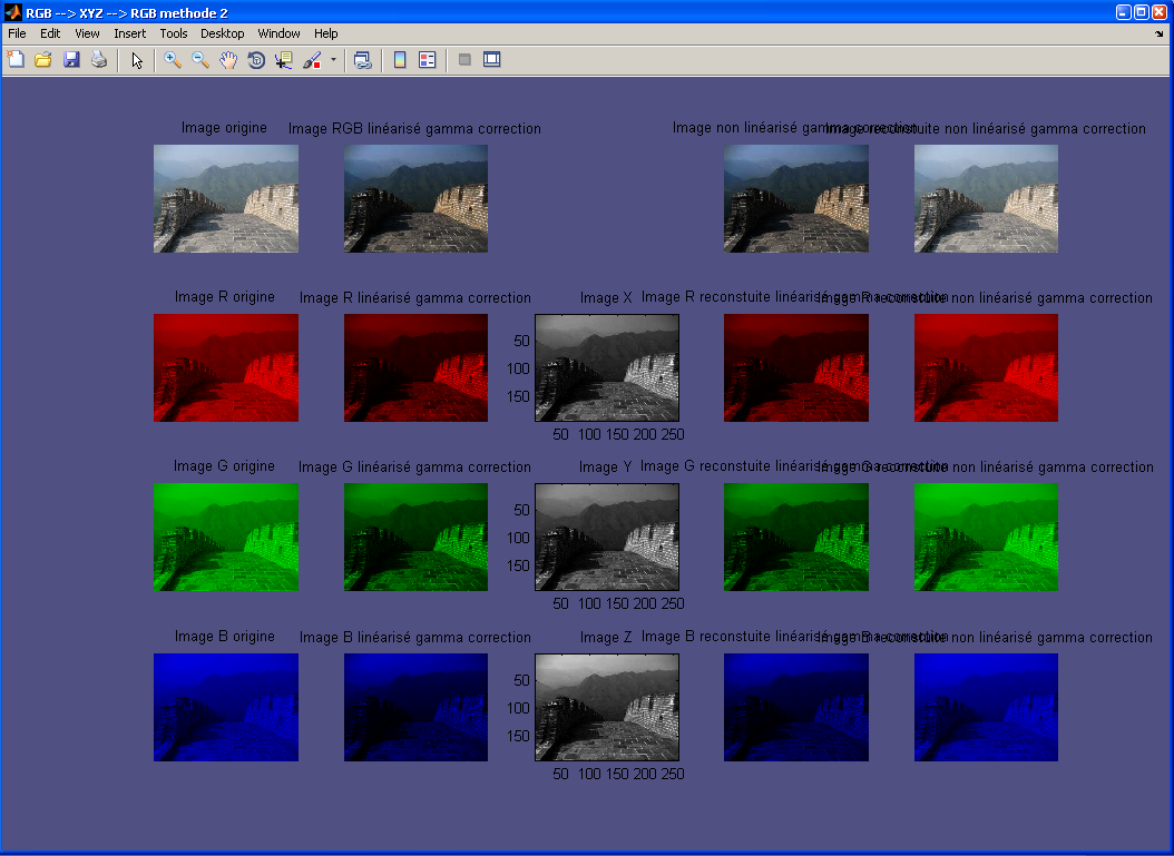
Copyright © 2010-2014, tous droits réservés, contact : operationpixel@free.fr